We took the proof-of-delivery workflow described in our POD processing benchmark, replaced the closed frontier models inside it with a combination of open-weight models, and re-ran the same 60 cases through the same scorer. The open-weight configuration scored 95.0 against 94.6 for the identical workflow on closed models, at 0.98× the cost. It is also roughly twice as slow.
Why this question matters now
Every finance team we talk to gets to the same question, usually in the first call: does our data have to leave our infrastructure for this to work? For a long time the honest answer was yes — or at least yes, if you want it to work well. The models that could reliably read a smudged delivery note were closed, and they all ran on somebody else's servers.
Open weights change that, and the useful part is how unglamorous the change is. You can download them and serve them on your own hardware. So it stops being a question of principle and becomes a question of price: what does the switch actually cost you?
We were able to check that directly. The workflow was already in production and the benchmark was already published, so the models were the only new variable.
What we changed, and what we did not
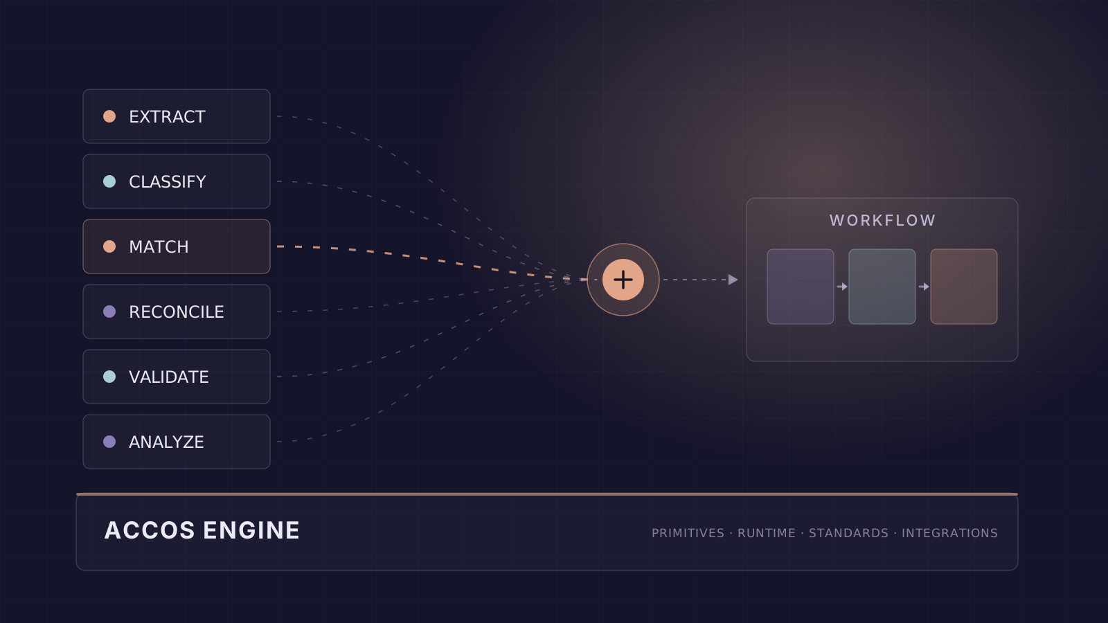
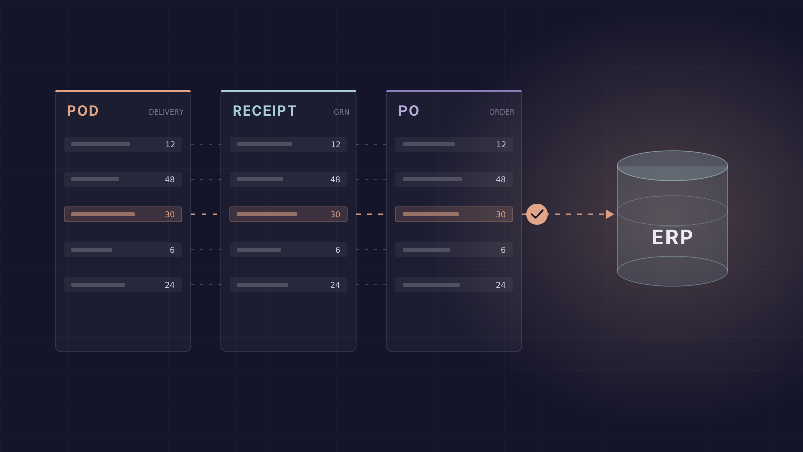
The models were the only thing we changed. The workflow is the same one that runs in our AP automation product: documents in, a reconciled invoice out, with a deterministic engine doing the matching and the arithmetic. The 60 cases are the same scanned proof-of-delivery, receipt-note and purchase-order sets. The scorer is the same composite, weighting line-item F1 at 0.70, line-field accuracy at 0.20 and header accuracy at 0.10.
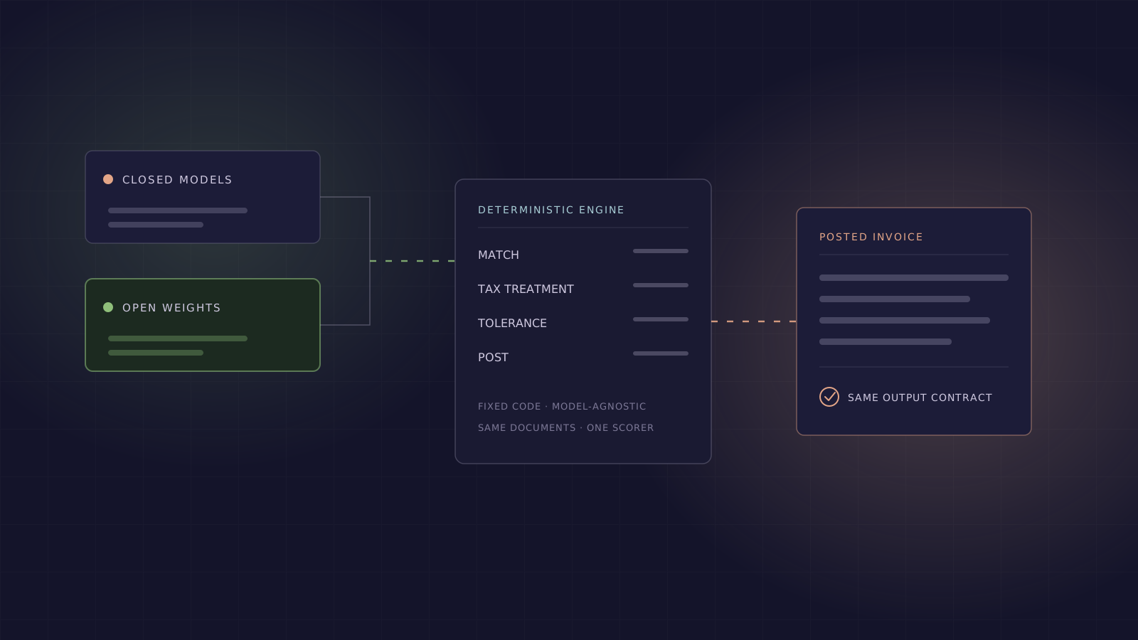
Inside the workflow, the model roles were repointed to a combination of open-weight models, including Kimi K3 and GLM. Which model serves which step is an implementation detail that changes as models improve, and we are not treating it as the result here. The swap is only possible because everything downstream of the reading step is fixed code, and that code does not care which model produced the numbers.
Results
What the numbers say
Accuracy barely moved. The two model classes sit half a point apart in Figure 1, and both sit more than a point clear of the best coding agent, so on this task the way the work is organised carries more weight than the choice of model. Cost came out level too, and the open-weight figure includes work redone after provider connection failures during the run, so a clean pass would come in lower; how far that generalises is covered under Limitations.
For teams whose blocker is data leaving their network, this is the part that matters. That option used to carry an accuracy penalty. On our workflow, using open source models did not cost us on accuracy.
The price of the swap: latency
Open-weight models are served by inference providers whose throughput and queueing behaviour differ from those of the large closed vendors. Across our runs the open-weight configuration takes on the order of twice as long per case as the closed-model configuration for an equivalent score.
The trade-off is fairly simple: you get data control without paying much more, but you wait longer. For an overnight batch, that probably doesn't matter. For someone sitting in front of an AP queue, it probably does.
How we measured
- Data. 60 cases from a public synthetic set, no customer data. Scanned, image-only proof-of-delivery documents, with their receipt notes and purchase orders. The same set used in our POD benchmark, so the numbers are directly comparable to the ones published there.
- Only the models changed. The workflow, the documents and the output contract are untouched, and the closed-model and coding-agent rows are reused unchanged from the earlier published run.
- Cost is measured, not estimated. Total LLM spend to complete all 60 cases, counted from token usage at provider list prices, expressed as a multiple of the closed-model configuration's spend.
- Latency is an approximate figure, not a benchmark result. This run's wall clock was taken on a shared machine, so we quote it roughly rather than pretending to a precise multiple.
One scorer grades every system. It is a weighted composite, computed per case and then averaged across the 60:
| Component | Weight | What it measures |
|---|---|---|
| Line-item F1 | 0.70 | whether the right set of delivered lines was found, penalising invented lines as well as missed ones |
| Line-field accuracy | 0.20 | whether the values on each matched line are right |
| Header accuracy | 0.10 | invoice number, dates, vendor, totals and the other document-level fields |
Limitations
Cost parity is workload-dependent, and this is the most important caveat on the page. Proof-of-delivery processing spends most of its tokens reading pages, with comparatively little multi-step reasoning per case. On a task weighted the other way, we have measured the same swap costing materially more than the closed-model configuration for an equivalent score. The 0.98× belongs to this workload only, and any team considering the switch should measure it on their own document mix.
This is one run of 60 cases. The accuracy figures in Figure 1 are means over 60 cases, one run per system, which is the same basis the earlier published comparison used. Repeat-stability across identical reruns is being measured separately and is not claimed here. In our earlier POD work that measure separated configurations more sharply than accuracy did, so its absence is a real gap in this page.
Provider reliability was visibly worse. The open-weight run lost extractions to repeated bursts of connection failures against the inference provider, and those documents had to be re-processed before the run was complete. Accuracy was unaffected, since a document either gets read or gets retried, but the operational difference between a mature closed API and the current open-weight serving landscape showed up clearly in the run logs.
What a given Cadel deployment looks like is a separate conversation. An open-weight model can run on infrastructure you control, but that says nothing about how any particular deployment of ours is actually configured. If you are solving for data residency, ask us about the specific arrangement; this benchmark does not settle it.
What comes next
We will re-run this as the open-weight models move, on the same harness and the same scorer, because a result like this has a shelf life measured in months. Two gaps still remain to explore: the first is repeat stability across runs, to prove the Cadel workflow has less variance than the agentic arms, and similarly, the second is measuring the mean latency to understand if our numbers could be a one-off result.
We treat the model layer under Cadel AP automation as a configuration choice. If data control is a constraint for your team, get in touch.